Trees in Data Structure Explained in 5 Minutes

Data is the most vital entity in Machine Learning and Data Science. And most times, this data can be present in the most complex and confusing form. There is, therefore, the need to always bring some order into the data.

Currently, a data structure is the most effective way to organize data so that it can effectively be put to use. And this data structuring can either be done linearly through the use of methods such as Arrays, Linked Lists, Stacks, and Queues or non-linearly through methods such as Graphs, Heaps, and Trees data structure.

Briefly, we will be looking at this last method to see what it means and learn how to do a binary tree implementation.

What “Trees in Data Structure” Means

Trees in data structure refer to a non-linear data representation comprising of connected nodes. The connections imply a relationship between the nodes and could be done through directed or undirected edges.

Each node contains an integer or value, which is how data is stored in the tree. To help you understand this better, imagine an actual family tree comprising of the grandparents, the parents, and their children.

The grandparents here would represent the root node. Data structures trees have a root node (the original and first node) with no known parents and, as a rule, only one root node may exist per tree.

The parents would represent every other subsequent node joined to the root node. And computer science trees usually have parent nodes that may or may not have children.

Lastly, the tree in the data structure also has children like an actual family would. A child node is a node joined to a parent. A child node may even have other children nodes of its own. A child node without children is termed a leaf or an external node, while those with children are called internal nodes.

Also, when a group of nodes stem from the same parent, we call such nodes siblings.

Arranged this way, these tree data structures give us the luxury of storing data hierarchically, and this can, in turn, save us a lot of time and effort when sorting and searching the data.

Types of Trees in Data Structures

There are three major types of trees data structures, namely:

A General Tree

In a general tree data structure, there are usually no restrictions on how many children a parent node can have. Each node can have zero or multiple children, and there are no rules for assigning nodes.

Most of the types of trees in computer science are available trees, with a prevalent example being the computer filing systems.

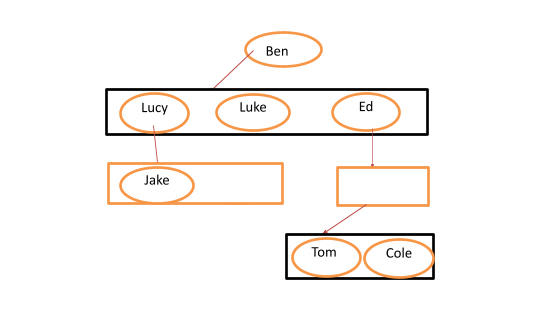
Because the number of nodes a parent node can later have is usually unknown from the start, we typically implement a general tree using the first child/next sibling method.

This works by assigning a new node to the far left and far right current nodes like in the diagram below:

Binary Tree

Many of us already know that the word “binary” means “not more than two.” Therefore, a binary tree is a tree with not more than two child nodes; one left child and one right child, as in the example below:

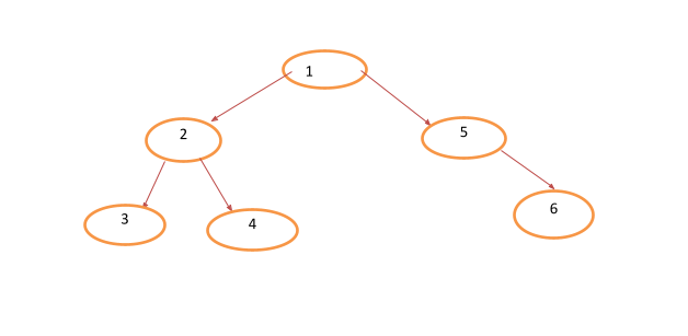
It is this type of arrangement that makes it easy to store and search for data so that computer operations such as data storage, insertion, discovery, and deletions can be done as quickly as possible. There are three components of every binary tree:

• Data or value
• Left child pointer
• Right child pointer

Binary Search Tree

This is perhaps the most orderly when we are considering the types of trees in a data structure. A binary search tree or BST is a type of tree that stores data in a well-sorted fashion so that lookups and other kinds of operations can be quickly done.

A characteristic feature of these types of trees in a data structure is that the integer in the top node is always bigger than the integer contained within the left child but smaller than the integer contained within the right child. Check the image below to get a better understanding.

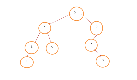
A closer look at the tree above shows the values in the rightmost nodes higher than its parent node, and the leftmost nodes’ values being lesser.

Tutorial on Binary Tree Implementation

We now know what a binary tree means. Next, let’s learn how to represent and implement it. So, we will take you through the steps and process involved in initializing a simple binary tree.

But first, we will use the code below to call our binary tree class:

class BinaryTree:
    def __init__(self, value):
        self.value = value
        self.left_child = None
        self.right_child = None

Both the left and right child are set to None because we are yet to pass values into them. We will then test the code using a value “a.”

tree = BinaryTree('a')
print(tree.value) # a
print(tree.left_child) # None
print(tree.right_child) # None

Next, we will begin to insert nodes. Let’s start with the nodes to the left side.

def insert_left(self, value):
    if self.left_child == None:
        self.left_child = BinaryTree(value)
    else:
        new_node = BinaryTree(value)
        new_node.left_child = self.left_child
        self.left_child = new_node

Then the nodes to our right.

def insert_right(self, value):
    if self.right_child == None:
        self.right_child = BinaryTree(value)
    else:
        new_node = BinaryTree(value)
        new_node.right_child = self.right_child
        self.right_child = new_node

Once this is done, our next task would be to build the binary tree by assigning values to each node. The code to do this is given below:

a_node = BinaryTree('a')
a_node.insert_left('b')
a_node.insert_right('c')

b_node = a_node.left_child
b_node.insert_right('d')

c_node = a_node.right_child
c_node.insert_left('e')
c_node.insert_right('f')

d_node = b_node.right_child
e_node = c_node.left_child
f_node = c_node.right_child

print(a_node.value) # a
print(b_node.value) # b
print(c_node.value) # c
print(d_node.value) # d
print(e_node.value) # e
print(f_node.value) # f

And once we have completed our binary tree, we can go ahead and traverse or search for a specific value. There are two options for traversing; Depth-First Search (DFS) or Breadth-First Search (BFS).

Depth-First Search: DFS is a tree algorithm used for searching for a defined value contained within trees in computer science. And usually, we start from the root node and search down to the leaves, one branch at a time. Every time we get to the end of that branch, we backtrack to search for the next branch.

We will use the diagram below to understand how DFS is done.

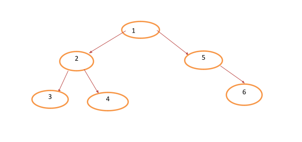
The result of a DFS search through the above tree would be 1-2-3-4-5-6.

There are three ways to conduct a DFS traversal; pre-order, in-order, and post-order searches.

Pre-order DFS: The process is as described above. The search starts from the root node, heads down on the left node, reaches the leaf, backtrack to search the next node until it gets to the rightmost node.

The code for pre-order search is given below:

def pre_order(self):
    print(self.value)

    if self.left_child:
        self.left_child.pre_order()

    if self.right_child:
        self.right_child.pre_order()

In-order DFS: this search starts from the leaf on the leftmost node first then heads to the middle nodes before finishing with the rightmost nodes. Let’ search through the tree below:

The result of this traversal would be 3-2-4-1-5-6. And the code is given below:

def in_order(self):
    if self.left_child:
        self.left_child.in_order()

    print(self.value)

    if self.right_child:
        self.right_child.in_order()

Post-order DFS: this starts from the left nodes, moves through the right nodes, and finishes last with the middle or upper nodes.

The traversal result for the above tree would be 3-4-2-6-5-1 and the code for it is given below:

def post_order(self):
    if self.left_child:
        self.left_child.post_order()

    if self.right_child:
        self.right_child.post_order()

    print(self.value)

Breadth-First Search: BFS, as a traversal algorithm, usually searches through each level before moving to the next level. Let’s look at the tree below,

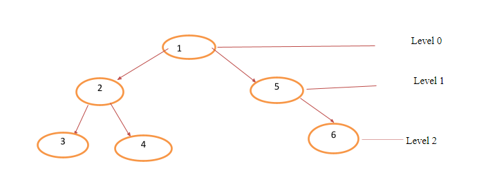
A BFS will first search through level 0, move to level 1, and finish off at level The results for the search would be 1-2-5-3-4-6, and we can write the algorithm with the code below:

def bfs(self):
    queue = Queue()
    queue.put(self)

    while not queue.empty():
        current_node = queue.get()
        print(current_node.value)

        if current_node.left_child:
            queue.put(current_node.left_child)

        if current_node.right_child:
            queue.put(current_node.right_child)

Trees in Data Science: Application and Importance

Trees in data science are sometimes called decision trees with useful application in predictive modeling, where they are used for practical approaches to different problems. 

Some of the other areas where trees data structure can be applied include:

• In customer relationship management, where online behaviors are used to predict a company’s income
• In business management, where customer’s deception can be detected and recognized in time
• In engineering and energy consumption, where faults can be predicted and remedied promptly
• In healthcare management, where data and results from previous tests can be used to foresee outcomes and provide better services for patients

In addition to this, there is much importance in using trees in data science, and some of them are:

• It naturally stores data in a hierarchical order making data storage less complex
• Unlike linear data structures, a binary tree can save us a lot of time
• With these trees, especially the general trees, there is no limit to how much nodes and data we can add
• The insertion/deletion function present, especially in a binary search tree, makes it easier to work with a large amount of data 

Conclusion

Data is essential for making informed decisions in today’s world, and the faster these decisions can be made, the better for everyone involved. While many types of data structures try to lighten the burden for data scientists, none does this quicker than trees data structure.

But the learning does not end here, so subscribe to our email newsletter to stay informed and to have a first peek at any new knowledge. Also, remember to share this value with all your friends.